English | 简体中文

Particle Filter Localization

A MATLAB implementation of particle filter localization for a mobile robot that measures its distance to known landmarks.

1 How the algorithm works

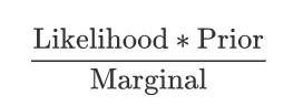
Particle filter localization is an application of Bayes' rule:

The walkthrough below follows the MATLAB code (particle_filter_localization.m).

1. Initialization
   1. Create a set of particles. The code uses NP=50, so there are 50 sample particles. Each particle is an estimated state [x y yaw] with 3 values: px=repmat(xEst,1,NP);
   2. Set the initial weights with pw=zeros(1,NP)+1/NP;, so every particle starts with the same weight.
   3. Place the landmarks with landMarks=[10 0; 10 10; 0 15; -5 20];, which gives 4 landmarks.
2. Prediction: use the motion model and the control input u to predict where each particle will be at the next time step.
   1. doControl() takes time and returns the control input u.
   2. doMotion() takes a state x and the control input u and returns the state at the next time step.
   3. doObservation() takes xGnd (the ground-truth pose, no noise), xOdom (the odometry estimate, with noise), u, landMarks and MAX_RANGE, and returns z, xGnd, xOdom, u.
3. Update: compute each particle's weight from the robot's observations z and the map values zl. A particle whose predicted observations are more similar to the actual landmark measurements gets a higher weight.
   1. Loop over every particle.
   2. Call doMotion() with the particle's state and the control input to get its state at the next time step, then add noise.
   3. Compute the weight as the product of Gaussian probabilities of the distance to each landmark.
4. Resampling: draw a new set of particles according to the weights w.

2 Key code

2.1 Observation model

% do Observation model 
function [z, xGnd, xOdom, u] = doObservation(xGnd, xOdom, u, landMarks, MAX_RANGE)
    global Qsigma;
    global Rsigma;
    
    % Gnd Truth and Odometry
    xGnd=doMotion(xGnd, u);% Ground Truth (ideal, noise-free)
    u=u+sqrt(Qsigma)*randn(2,1); % add noise randomly
    xOdom=doMotion(xOdom, u); % odometry only
    
    %Simulate Observation
    z=[];
    for iz=1:length(landMarks(:,1))
        dx = xGnd(1)-landMarks(iz,1);
        dy = xGnd(2)-landMarks(iz,2);
        d=sqrt(dx^2+dy^2);
        if d<MAX_RANGE 
            z=[z;[d+sqrt(Rsigma)*randn(1,1) landMarks(iz,:)]];   % add observation noise randomly
        end
    end
end

2.2 Motion model

% do Motion Model
function [ x ] = doMotion( x, u)
    global dt;
    Delta = [ [dt*cos(x(3)),0];
              [dt*sin(x(3)),0];
              [0,dt]];

    x = x+Delta*u;
end

2.3 Gaussian function

% Gauss function
function g = Gaussian(x,u,sigma)
    g=exp(-((u-x)^2)/(sigma^2)/2.0)/sqrt(2.0*pi*(sigma^2));
end

2.4 Weight normalization

% Normalization 
function pw=Normalization(pw,NP)
    pw=pw/sum(pw);

end

2.5 Resampling

function [px,pw]=ResamplingStep(px,pw,NTh,NP)
    ww=pw(1);
    for iw=2:NP
        ww=[ww,ww(end)+pw(iw)];
    end
    pw1=[]
    pp=[];
    for i=1:NP
        r=rand();
        for j=1:NP
            if ww(j)>r
                pp=[pp,px(:,j)]; 
                pw1=[pw1,pw(:,j)]
                break
            end
        end
    end
    px=pp;
    pw=pw1;
end

3 Experiments with the number of particles

3.1 Results for different NP

NP	Result	Run time (s)
3		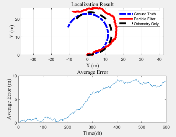0.220
5		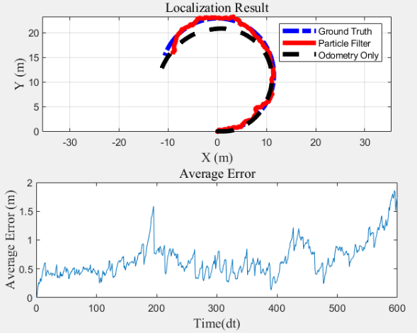0.286
10		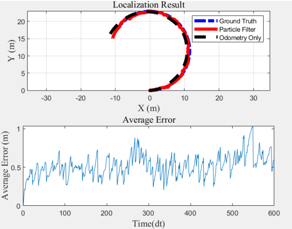0.387
25		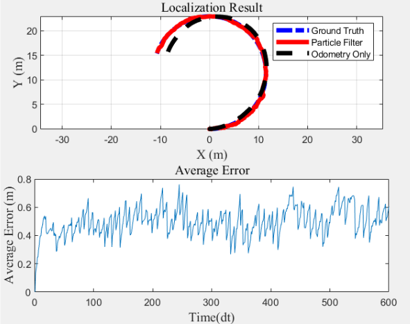0.640
50		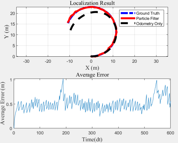1.131
100		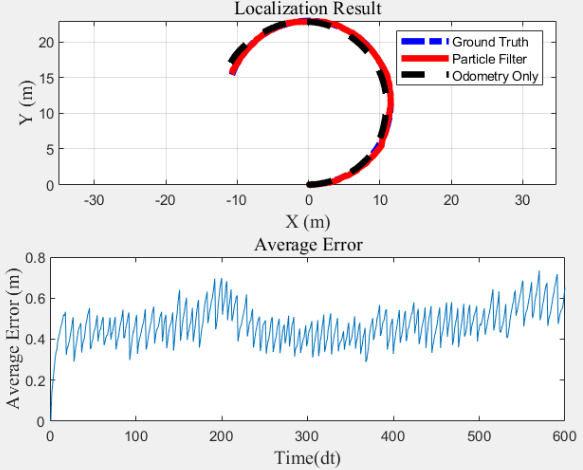2.159

3.2 Effect of NP on run time

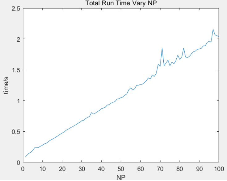
Run time grows linearly with the number of particles.

3.3 Effect of NP on error

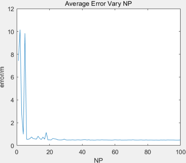
The error levels off at about 0.5, mainly because of the Gaussian noise.

4 Conclusions

The particle filter is a probabilistic localization method. Its strengths:

• It is easy to understand: the more similar a particle is to the observations, the more likely it is to survive.
• It is cheap to compute: the cost grows linearly with the number of particles.

Its weaknesses:

• It depends heavily on the initial state estimate. A poor choice can make it diverge.
• It needs fixed landmarks.

References

https://en.wikipedia.org/wiki/Particle_filter

Sebastian Thrun, Wolfram Burgard and Dieter Fox, Probabilistic Robotics